Time series forecasting involves predicting future values based on historical data. This article will focus on the ARIMA (Auto-Regressive Integrated Moving Average) forecasting models. We’ll do a walk through on implementing the models in Python, using the given dataset to forecast incoming calls.
Setting Up Your Environment
Before diving into the code, create a virtual environment to keep your project dependencies isolated.
On Windows:
python -m venv arima_env
.\arima_env\Scripts\activate
pip install pandas matplotlib statsmodels
On Linux:
python3 -m -venv arima_env
source arima_env/bin/activate
pip install pandas matplotlib statsmodels
statsmodels installs scipy compiled from source, which can take a few minutes. Just give it time and it will install.
Save the data below as: call_center_data.csv in the root folder.
Index,Incoming Calls,Answered Calls,Answer Rate,Abandoned Calls,Answer Speed (AVG),Talk Duration (AVG),Waiting Time (AVG),Service Level (20 Seconds)
1,217,204,94.01%,13,0:00:17,0:02:14,0:02:45,76.28%
2,200,182,91.00%,18,0:00:20,0:02:22,0:06:55,72.73%
3,216,198,91.67%,18,0:00:18,0:02:38,0:03:50,74.30%
4,155,145,93.55%,10,0:00:15,0:02:29,0:03:12,79.61%
5,37,37,100.00%,0,0:00:03,0:02:06,0:00:35,97.30%
6,315,304,96.51%,11,0:00:18,0:01:35,0:02:37,77.17%
7,252,244,96.83%,8,0:00:13,0:01:50,0:02:02,82.00%
8,213,205,96.24%,8,0:00:10,0:02:10,0:03:22,88.10%
9,219,200,91.32%,19,0:00:15,0:02:18,0:06:12,79.45%
10,371,348,93.80%,23,0:00:19,0:01:40,0:03:29,73.63%
11,166,164,98.80%,2,0:00:12,0:02:10,0:02:46,81.33%
12,32,32,100.00%,0,0:00:02,0:02:03,0:00:03,100.00%
13,231,222,96.10%,9,0:00:08,0:01:49,0:02:18,86.46%
14,205,197,96.10%,8,0:00:07,0:01:52,0:02:48,92.61%
15,338,313,92.60%,25,0:00:13,0:01:51,0:03:40,80.06%
16,180,174,96.67%,6,0:00:13,0:02:18,0:03:26,83.80%
17,226,211,93.36%,15,0:00:20,0:02:04,0:04:53,76.23%
18,226,212,93.81%,14,0:00:10,0:02:03,0:02:45,84.44%
19,45,44,97.78%,1,0:00:02,0:02:04,0:00:55,97.78%
20,218,194,88.99%,24,0:00:26,0:02:43,0:06:28,68.98%
21,187,174,93.05%,13,0:00:15,0:02:16,0:04:39,81.52%
22,191,184,96.34%,7,0:00:10,0:02:09,0:03:40,85.64%
23,188,174,92.55%,14,0:00:15,0:02:25,0:03:09,76.88%
24,154,148,96.10%,6,0:00:10,0:02:27,0:03:36,85.06%
25,166,150,90.36%,16,0:00:18,0:02:26,0:04:38,76.83%
26,58,57,98.28%,1,0:00:04,0:02:26,0:00:58,94.83%
27,160,153,95.63%,7,0:00:10,0:02:23,0:02:45,84.91%
28,86,79,91.86%,7,0:00:32,0:02:43,0:04:40,61.63%
29,180,170,94.44%,10,0:00:23,0:02:31,0:05:45,77.53%
30,210,192,91.43%,18,0:00:26,0:02:16,0:05:35,67.46%
31,163,157,96.32%,6,0:00:14,0:02:19,0:02:55,81.37%
32,143,140,97.90%,3,0:00:15,0:02:20,0:04:43,82.52%
33,57,55,96.49%,2,0:00:06,0:02:03,0:01:50,91.23%
34,179,172,96.09%,7,0:00:13,0:02:17,0:03:23,82.49%
35,194,184,94.85%,10,0:00:24,0:02:24,0:03:19,70.10%
36,201,196,97.51%,5,0:00:15,0:02:16,0:04:53,81.59%
37,218,189,86.70%,29,0:00:32,0:02:37,0:08:04,57.41%
38,194,190,97.94%,4,0:00:16,0:02:22,0:02:02,81.77%
39,227,219,96.48%,8,0:00:15,0:02:44,0:03:55,83.63%
40,52,52,100.00%,0,0:00:09,0:02:16,0:00:52,94.23%
41,385,370,96.10%,15,0:00:20,0:02:11,0:03:10,76.19%
42,137,130,94.89%,7,0:00:16,0:02:26,0:09:47,75.91%
43,254,252,99.21%,2,0:00:10,0:02:08,0:01:10,91.34%
44,211,206,97.63%,5,0:00:11,0:02:24,0:04:37,87.14%
45,282,279,98.94%,3,0:00:07,0:02:18,0:01:11,93.21%
46,262,260,99.24%,2,0:00:08,0:02:31,0:01:13,90.80%
47,65,63,96.92%,2,0:00:12,0:02:22,0:02:10,85.94%
48,325,323,99.38%,2,0:00:05,0:02:13,0:01:14,96.90%
49,235,230,97.87%,5,0:00:05,0:02:19,0:00:58,96.14%
50,215,212,98.60%,3,0:00:05,0:02:14,0:00:58,95.81%
51,85,85,100.00%,0,0:00:03,0:02:26,0:00:55,97.65%
52,195,195,100.00%,0,0:00:05,0:02:24,0:02:13,97.44%
53,188,182,96.81%,6,0:00:15,0:02:14,0:01:51,83.61%
54,58,58,100.00%,0,0:00:06,0:02:22,0:00:52,94.83%
55,251,247,98.41%,4,0:00:14,0:02:16,0:01:53,83.53%
56,181,178,98.34%,3,0:00:12,0:02:24,0:01:57,86.19%
57,228,213,93.42%,15,0:00:26,0:02:16,0:03:07,63.56%
58,165,163,98.79%,2,0:00:09,0:02:25,0:02:20,90.24%
59,185,179,96.76%,6,0:00:17,0:02:17,0:02:33,78.57%
60,172,164,95.35%,8,0:00:18,0:02:27,0:04:09,77.06%
61,57,51,89.47%,6,0:00:07,0:01:47,0:03:40,90.57%
62,200,192,96.00%,8,0:00:10,0:02:18,0:02:49,86.43%
63,202,199,98.51%,3,0:00:08,0:02:05,0:01:17,91.00%
64,217,212,97.70%,5,0:00:07,0:01:55,0:01:50,94.42%
65,225,223,99.11%,2,0:00:09,0:02:09,0:01:06,91.93%
66,235,231,98.30%,4,0:00:08,0:02:19,0:01:06,95.71%
67,202,201,99.50%,1,0:00:08,0:02:21,0:01:53,94.55%
68,43,39,90.70%,4,0:00:11,0:02:15,0:01:50,76.19%
69,194,187,96.39%,7,0:00:10,0:02:27,0:02:30,87.43%
70,202,199,98.51%,3,0:00:13,0:02:23,0:01:58,86.07%
71,146,140,95.89%,6,0:00:12,0:02:13,0:04:35,83.45%
72,147,145,98.64%,2,0:00:09,0:02:15,0:00:58,91.16%
73,155,145,93.55%,10,0:00:12,0:02:33,0:04:33,82.24%
74,157,156,99.36%,1,0:00:09,0:02:24,0:00:53,92.95%
75,38,36,94.74%,2,0:00:13,0:02:11,0:00:59,83.78%
76,166,162,97.59%,4,0:00:09,0:02:29,0:02:45,89.09%
77,226,216,95.58%,10,0:00:13,0:02:15,0:01:46,81.45%
78,253,247,97.63%,6,0:00:10,0:01:54,0:01:17,88.49%
79,134,134,100.00%,0,0:00:03,0:02:13,0:00:26,100.00%
80,70,67,95.71%,3,0:00:12,0:02:01,0:01:16,83.82%
81,83,82,98.80%,1,0:00:07,0:02:03,0:01:16,95.18%
82,42,40,95.24%,2,0:00:08,0:01:51,0:01:36,90.24%
83,66,64,96.97%,2,0:00:05,0:02:00,0:01:39,95.45%
84,153,146,95.42%,7,0:00:20,0:02:08,0:04:32,76.00%
85,141,135,95.74%,6,0:00:23,0:02:06,0:02:15,66.91%
86,146,143,97.95%,3,0:00:17,0:01:57,0:02:27,78.32%
87,144,140,97.22%,4,0:00:12,0:01:53,0:02:05,84.03%
88,105,103,98.10%,2,0:00:17,0:01:55,0:02:01,76.19%
89,36,35,97.22%,1,0:00:16,0:01:54,0:01:31,77.14%
90,61,57,93.44%,4,0:00:04,0:02:00,0:03:41,91.67%
91,60,58,96.67%,2,0:00:11,0:02:08,0:01:34,85.00%
92,18,17,94.44%,1,0:00:05,0:02:39,0:00:20,100.00%
93,206,202,98.06%,4,0:00:09,0:01:54,0:01:10,89.27%
94,194,193,99.48%,1,0:00:11,0:01:57,0:01:34,84.97%
95,206,200,97.09%,6,0:00:10,0:02:08,0:02:00,86.27%
96,53,53,100.00%,0,0:00:18,0:02:08,0:02:10,77.36%
97,147,145,98.64%,2,0:00:09,0:01:50,0:01:24,88.36%
98,201,197,98.01%,4,0:00:09,0:01:59,0:02:23,90.95%
99,202,198,98.02%,4,0:00:10,0:02:09,0:01:11,88.50%
100,226,219,96.90%,7,0:00:10,0:02:12,0:02:45,88.00%
101,167,163,97.60%,4,0:00:07,0:02:09,0:01:50,92.77%
102,164,164,100.00%,0,0:00:11,0:02:17,0:01:45,89.02%
103,42,41,97.62%,1,0:00:11,0:02:09,0:01:18,87.80%
104,79,78,98.73%,1,0:00:07,0:02:23,0:00:48,94.87%
105,165,162,98.18%,3,0:00:09,0:02:09,0:01:50,89.70%
106,180,174,96.67%,6,0:00:16,0:02:16,0:01:43,77.78%
107,179,176,98.32%,3,0:00:10,0:02:26,0:01:50,87.64%
108,217,215,99.08%,2,0:00:08,0:02:08,0:02:07,91.71%
109,171,167,97.66%,4,0:00:10,0:02:15,0:01:50,86.47%
110,37,37,100.00%,0,0:00:09,0:01:57,0:01:22,86.49%
111,215,206,95.81%,9,0:00:18,0:02:09,0:02:45,80.95%
112,218,212,97.25%,6,0:00:16,0:02:17,0:02:09,84.26%
113,205,202,98.54%,3,0:00:11,0:02:25,0:01:37,90.69%
114,195,190,97.44%,5,0:00:12,0:02:22,0:01:14,89.01%
115,181,176,97.24%,5,0:00:13,0:02:13,0:01:16,82.22%
116,212,206,97.17%,6,0:00:11,0:02:20,0:01:49,89.42%
117,33,32,96.97%,1,0:00:08,0:02:28,0:00:55,90.91%
118,298,287,96.31%,11,0:00:13,0:01:35,0:02:51,83.33%
119,158,156,98.73%,2,0:00:11,0:02:23,0:01:32,89.81%
120,156,154,98.72%,2,0:00:12,0:02:13,0:01:01,85.81%
121,163,163,100.00%,0,0:00:10,0:02:02,0:02:46,92.64%
122,98,98,100.00%,0,0:00:07,0:02:10,0:01:10,93.88%
123,255,249,97.65%,6,0:00:15,0:02:19,0:05:31,82.68%
124,50,49,98.00%,1,0:00:08,0:02:02,0:00:57,92.00%
125,290,289,99.66%,1,0:00:12,0:02:01,0:01:10,89.27%
126,296,281,94.93%,15,0:00:22,0:02:08,0:04:30,73.54%
127,260,257,98.85%,3,0:00:17,0:02:13,0:01:20,87.16%
128,201,193,96.02%,8,0:00:19,0:02:23,0:02:02,76.77%
129,132,131,99.24%,1,0:00:17,0:02:13,0:01:30,76.52%
130,167,165,98.80%,2,0:00:09,0:02:06,0:00:57,92.12%
131,85,79,92.94%,6,0:00:18,0:02:25,0:01:53,77.38%
132,244,236,96.72%,8,0:00:21,0:02:29,0:01:56,75.62%
133,186,182,97.85%,4,0:00:14,0:02:13,0:01:38,79.03%
134,278,264,94.96%,14,0:00:19,0:02:20,0:02:10,76.84%
135,272,268,98.53%,4,0:00:15,0:02:30,0:01:45,80.00%
136,218,206,94.50%,12,0:00:25,0:02:21,0:03:41,67.28%
137,152,148,97.37%,4,0:00:14,0:02:18,0:01:25,83.33%
138,48,43,89.58%,5,0:00:22,0:02:01,0:01:21,69.57%
139,186,181,97.31%,5,0:00:14,0:02:20,0:01:49,84.95%
140,182,180,98.90%,2,0:00:08,0:02:10,0:00:58,93.37%
141,192,188,97.92%,4,0:00:20,0:01:58,0:01:56,76.19%
142,155,148,95.48%,7,0:00:14,0:02:24,0:02:18,85.33%
143,144,142,98.61%,2,0:00:11,0:02:19,0:01:05,90.21%
144,164,162,98.78%,2,0:00:12,0:02:35,0:01:50,85.37%
145,27,26,96.30%,1,0:00:11,0:02:04,0:01:17,81.48%
146,177,175,98.87%,2,0:00:11,0:02:19,0:01:35,90.86%
147,134,131,97.76%,3,0:00:14,0:02:23,0:01:39,81.34%
148,125,120,96.00%,5,0:00:14,0:02:20,0:02:52,84.55%
149,167,163,97.60%,4,0:00:16,0:02:24,0:01:12,81.21%
150,169,167,98.82%,2,0:00:09,0:02:14,0:01:44,89.94%
151,162,160,98.77%,2,0:00:16,0:02:15,0:01:31,83.13%
152,25,25,100.00%,0,0:00:16,0:02:35,0:00:58,76.00%
153,157,146,92.99%,11,0:00:17,0:02:17,0:01:51,79.74%
154,166,154,92.77%,12,0:00:25,0:02:18,0:03:39,66.26%
155,58,55,94.83%,3,0:00:16,0:02:11,0:02:45,74.14%
156,75,74,98.67%,1,0:00:15,0:02:13,0:03:18,84.00%
157,28,28,100.00%,0,0:00:07,0:02:28,0:00:51,96.43%
158,108,107,99.07%,1,0:00:09,0:02:11,0:00:59,94.44%
159,21,21,100.00%,0,0:00:07,0:02:58,0:00:58,95.24%
160,189,182,96.30%,7,0:00:21,0:02:10,0:04:46,76.34%
161,161,155,96.27%,6,0:00:19,0:02:27,0:01:50,71.88%
162,155,151,97.42%,4,0:00:17,0:02:20,0:01:49,80.52%
163,161,150,93.17%,11,0:00:17,0:02:22,0:02:45,75.32%
164,132,129,97.73%,3,0:00:27,0:02:22,0:02:34,65.15%
165,122,119,97.54%,3,0:00:16,0:02:24,0:01:50,80.00%
166,17,17,100.00%,0,0:00:21,0:02:40,0:00:58,76.47%
167,45,45,100.00%,0,0:00:06,0:02:06,0:00:57,95.56%
168,177,172,97.18%,5,0:00:20,0:02:23,0:02:51,76.00%
169,133,132,99.25%,1,0:00:10,0:02:25,0:00:59,93.23%
170,177,167,94.35%,10,0:00:15,0:02:22,0:04:35,83.24%
171,127,124,97.64%,3,0:00:16,0:02:22,0:01:45,81.89%
172,148,147,99.32%,1,0:00:16,0:02:11,0:03:11,83.11%
173,23,23,100.00%,0,0:00:32,0:02:02,0:02:43,65.22%
174,141,134,95.04%,7,0:00:24,0:02:38,0:02:29,72.14%
175,124,120,96.77%,4,0:00:20,0:02:33,0:02:58,82.26%
176,165,156,94.55%,9,0:00:25,0:02:21,0:02:38,70.55%
177,168,166,98.81%,2,0:00:21,0:02:33,0:03:43,80.12%
178,198,188,94.95%,10,0:00:22,0:02:32,0:02:45,70.92%
179,139,133,95.68%,6,0:00:17,0:02:40,0:03:03,80.15%
180,46,45,97.83%,1,0:00:10,0:02:14,0:01:16,88.89%
181,184,174,94.57%,10,0:00:23,0:02:37,0:04:35,76.54%
182,207,190,91.79%,17,0:00:21,0:02:23,0:04:06,71.36%
183,191,180,94.24%,11,0:00:21,0:02:32,0:01:53,76.50%
184,213,204,95.77%,9,0:00:24,0:02:26,0:02:46,69.67%
185,483,451,93.37%,32,0:00:16,0:00:57,0:08:45,79.20%
186,547,526,96.16%,21,0:00:19,0:01:21,0:03:54,81.58%
187,54,53,98.15%,1,0:00:25,0:02:36,0:01:18,70.37%
188,275,261,94.91%,14,0:00:22,0:02:13,0:02:12,74.44%
189,205,195,95.12%,10,0:00:24,0:02:34,0:03:00,70.79%
190,80,77,96.25%,3,0:00:10,0:02:11,0:01:33,89.61%
191,200,195,97.50%,5,0:00:21,0:02:30,0:02:48,75.25%
192,154,150,97.40%,4,0:00:21,0:02:29,0:02:45,74.34%
193,163,155,95.09%,8,0:00:23,0:02:18,0:02:26,74.52%
194,12,12,100.00%,0,0:00:25,0:03:37,0:01:28,66.67%
195,218,212,97.25%,6,0:00:20,0:01:56,0:04:11,75.93%
196,172,163,94.77%,9,0:00:18,0:02:09,0:01:53,81.93%
197,205,194,94.63%,11,0:00:18,0:02:24,0:01:41,80.60%
198,178,168,94.38%,10,0:00:23,0:02:28,0:02:50,68.97%
199,214,201,93.93%,13,0:00:23,0:02:11,0:02:24,66.03%
200,169,161,95.27%,8,0:00:23,0:02:17,0:04:35,71.69%
Understanding ARIMA Models
ARIMA works by capturing patterns in historical data and projecting them into the future. This makes ARIMA especially useful for datasets where trends and seasonality affect the target variable.
In the context of a call center, forecasting is vital for managing resources and ensuring optimal service levels. For instance, predictions about the number of incoming calls help allocate staff efficiently. Accurate forecasts also help reduce abandoned calls and improve customer satisfaction. Using the dataset provided, which includes metrics like Incoming Calls, Answered Calls, and Answer Rate, an ARIMA model can predict future call volumes based on historical data.
How ARIMA Models Work
ARIMA operates on three main components:
- Auto-regression (AR): Relates to the dependency between an observation and a specified number of lagged observations.
- Integration (I): Refers to differencing the data to make it stationary. Stationarity implies that the statistical properties of the time series, such as mean and variance, are consistent over time.
- Moving Average (MA): Models the relationship between an observation and the residual errors from a moving average model applied to past observations.
The model’s parameters — p (lags in AR), d (degree of differencing), and q (lags in MA)—determine its structure.
Applying ARIMA to Call Center Data
The call center dataset includes daily incoming call counts, which we aim to forecast. Predictions can help answer questions like:
- How many calls should the center expect next week?
- Will there be a spike in calls during a particular day or time?
- How can staffing be adjusted to handle call volumes?
Preparing the Dataset in Python
Start by loading and preparing the data. We’ll focus on the Incoming Calls column for simplicity.
import pandas as pd

# Load the dataset
data = pd.read_csv("call_center_data.csv")  # Replace with your file path
data['Incoming Calls'] = pd.to_numeric(data['Incoming Calls'], errors='coerce')
data.dropna(inplace=True)

# Create a date range index
data.index = pd.date_range(start='1/1/2023', periods=len(data), freq='D')

# Inspect the data
print(data.head())
Expected result:
PS C:\arima> & C:/arima/arima_env/Scripts/python.exe c:/arima/arima.py
            Index  Incoming Calls  ...  Waiting Time (AVG) Service Level (20 Seconds)
2023-01-01      1             217  ...             0:02:45                     76.28%
2023-01-02      2             200  ...             0:06:55                     72.73%
2023-01-03      3             216  ...             0:03:50                     74.30%
2023-01-04      4             155  ...             0:03:12                     79.61%
2023-01-05      5              37  ...             0:00:35                     97.30%

[5 rows x 9 columns]
Visualizing the Time Series
Before applying ARIMA, visualize the data to identify trends or seasonality.
import pandas as pd
import matplotlib.pyplot as plt

# FIRST CODE: Load and preprocess the dataset
data = pd.read_csv("call_center_data.csv")  # Replace with your file path
data['Incoming Calls'] = pd.to_numeric(data['Incoming Calls'], errors='coerce')  # Ensure numerical data
data.dropna(inplace=True)  # Drop rows with missing values

# Create a date range index
data.index = pd.date_range(start='1/1/2023', periods=len(data), freq='D')

# Inspect the dataset
print(data.head())

# OTHER CODE: Visualize the data
plt.plot(data.index, data['Incoming Calls'])
plt.title("Daily Incoming Calls")
plt.xlabel("Date")
plt.ylabel("Incoming Calls")
plt.show()
Result:
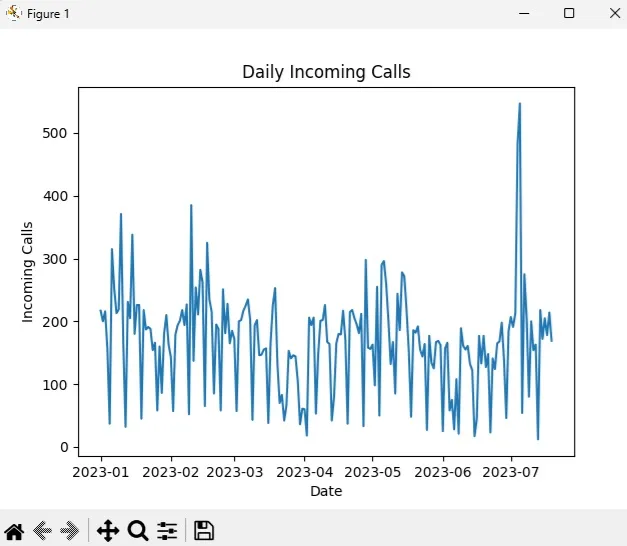
Visual Inspection from the Plot
Check for Trends:
- Look for an upward or downward slope in the data.
- In your plot, there may not be a clear trend over time, but there are fluctuations in magnitude.
Check for Seasonality:
- Look for repeating patterns or cycles at regular intervals.
- If seasonality exists, the time series may still need to be transformed or differenced.
Variance Consistency:
- Check if the variance (spread) of data points increases or decreases over time.
- If the variance is not constant, a log transformation or differencing may be required.
In the data and visualization above there is no clear Trend or Seasonality. There does appear to be two outliers (records 185 and 186), we’ll use Augmented Dickey-Fuller (ADF) below to see if differencing is needed:
185,483,451,93.37%,32,0:00:16,0:00:57,0:08:45,79.20%
186,547,526,96.16%,21,0:00:19,0:01:21,0:03:54,81.58%
Making the Data Stationary
Stationarity is a prerequisite for ARIMA. Use the Augmented Dickey-Fuller (ADF) test to check if the time series is stationary (has consistent statistical properties over time).
For example: you couldn’t mix daily and hourly call totals and expect ARIMA models to generate a useable forecast. Similarly, you couldn’t run the model’s using data that is incomplete (missing days or missing chunks of hourly data).
# Step 1: Load and clean the dataset
import pandas as pd
from statsmodels.tsa.stattools import adfuller
import matplotlib.pyplot as plt

data = pd.read_csv("call_center_data.csv")
data['Incoming Calls'] = pd.to_numeric(data['Incoming Calls'], errors='coerce')
data.dropna(inplace=True)

# Step 2: Visualize the time series
plt.plot(data.index, data['Incoming Calls'])
plt.title("Daily Incoming Calls")
plt.xlabel("Date")
plt.ylabel("Incoming Calls")
plt.show()

# Step 3: Perform the Augmented Dickey-Fuller (ADF) Test
result = adfuller(data['Incoming Calls'])
print("ADF Statistic:", result[0])
print("p-value:", result[1])

if result[1] < 0.05:
    print("The data is stationary.")
else:
    print("The data is not stationary. Differencing is needed.")
Stationary Result:
ADF Statistic: -3.225413025937688
p-value: 0.018560000445111382
The data is stationary.
Non-stationary Result:
ADF Statistic: -0.945
p-value: 0.560
The data is not stationary. Differencing is needed.
If the data isn’t stationary, apply differencing.
data['Incoming Calls Diff'] = data['Incoming Calls'].diff().dropna()Implementing the ARIMA Model
Now, fit an ARIMA model to the data. The statsmodels library provides tools for this.
Model Definition and Fitting
import pandas as pd
from statsmodels.tsa.arima.model import ARIMA
import matplotlib.pyplot as plt
# Load the dataset (assumes previous preprocessing)
data = pd.read_csv("call_center_data.csv")
data['Incoming Calls'] = pd.to_numeric(data['Incoming Calls'], errors='coerce')
data.dropna(inplace=True)
data.index = pd.date_range(start='1/1/2023', periods=len(data), freq='D')
# Define ARIMA model with chosen parameters (example: p=1, d=1, q=1)
model = ARIMA(data['Incoming Calls'], order=(1, 1, 1))
model_fit = model.fit()
# Print model summary
print(model_fit.summary())
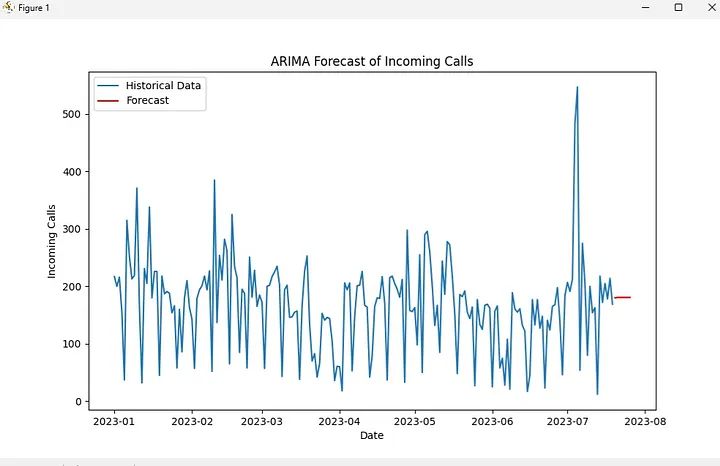
# Forecast the next 7 days
forecast = model_fit.forecast(steps=7)
# Visualize the forecast
plt.plot(data.index, data['Incoming Calls'], label="Historical Data")
forecast_index = pd.date_range(data.index[-1], periods=7, freq='D')
plt.plot(forecast_index, forecast, label="Forecast", color="red")
plt.title("ARIMA Forecast of Incoming Calls")
plt.xlabel("Date")
plt.ylabel("Incoming Calls")Expected Result:
(arima_env) PS C:\arima> & C:/arima/arima_env/Scripts/python.exe c:/arima/arima.py
                               SARIMAX Results
==============================================================================
Dep. Variable:         Incoming Calls   No. Observations:                  200
Model:                 ARIMA(1, 1, 1)   Log Likelihood               -1155.771
Date:                Tue, 19 Nov 2024   AIC                           2317.542
Time:                        18:34:25   BIC                           2327.422
Sample:                    01-01-2023   HQIC                          2321.541
                         - 07-19-2023
Covariance Type:                  opg
==============================================================================
                 coef    std err          z      P>|z|      [0.025      0.975]
------------------------------------------------------------------------------
ar.L1          0.0648      0.067      0.974      0.330      -0.066       0.195
ma.L1         -0.9094      0.034    -26.510      0.000      -0.977      -0.842
sigma2      6436.6671    477.593     13.477      0.000    5500.601    7372.733
===================================================================================
Ljung-Box (L1) (Q):                   0.01   Jarque-Bera (JB):                52.64
Prob(Q):                              0.92   Prob(JB):                         0.00
Heteroskedasticity (H):               1.23   Skew:                             0.46
Prob(H) (two-sided):                  0.40   Kurtosis:                         5.34
===================================================================================

Warnings:
[1] Covariance matrix calculated using the outer product of gradients (complex-step).
That output is a summary of the ARIMA(1, 1, 1) model fitted to Incoming Calls data. Here’s a detailed explanation of each part:
1. Model Overview
Dep. Variable: Incoming Calls – The target variable being modeled.
No. Observations: 200 – The number of data points used in the model.
Model: ARIMA(1, 1, 1) – Specifies the ARIMA configuration:
p=1 (1 autoregressive term).
d=1 (1 differencing applied to make the data stationary).
q=1 (1 moving average term).
Log Likelihood: -1155.771 – A measure of model fit. Higher (less negative) values indicate better fit.
AIC (Akaike Information Criterion): 2317.542 – A measure used to compare models. Lower values indicate a better model fit with fewer parameters.
BIC (Bayesian Information Criterion): 2327.422 – Similar to AIC but penalizes models with more parameters more heavily.
HQIC: 2321.541 – Another criterion for model selection, similar to AIC and BIC.
2. Model Coefficients
ar.L1 (Autoregressive Lag 1): 0.0648 – Coefficient for the AR(1) term. A small value here indicates weak dependence on the first lag.
P>|z| = 0.330: The p-value for this coefficient. Since it’s >0.05, this term may not be statistically significant.
a.L1 (Moving Average Lag 1): -0.9094 – Coefficient for the MA(1) term. A value close to -1 suggests strong negative correlation with the lagged forecast errors.
P>|z| = 0.000: This term is statistically significant (p-value < 0.05).
sigma2: 6436.6671 – The variance of the residuals (forecast errors). Higher values indicate more variability in the forecast.
3. Diagnostics
Ljung-Box Test (Q): Tests whether residuals (errors) are uncorrelated.
Prob(Q) = 0.92: Since the p-value is high (>0.05), there is no significant autocorrelation in the residuals.
Jarque-Bera (JB): Tests whether residuals are normally distributed.
Prob(JB) = 0.00: A low p-value suggests the residuals deviate significantly from normality.
Heteroskedasticity (H): Tests whether residual variance is constant.
Prob(H) = 0.40: A high p-value suggests no significant heteroskedasticity (variance appears stable).
4. Warnings
- Covariance Matrix: The warning indicates that the covariance matrix for the coefficients was estimated using the “outer product of gradients” method. This is not a problem but may suggest numerical complexities in estimating standard errors.
What This Tells You
Fit Quality:
- The model appears to fit the data well enough to continue, as indicated by the high significance of the
ma.L1term and the lack of residual autocorrelation (Ljung-Box test). - However, the
ar.L1term is not statistically significant, so you could consider simplifying the model toARIMA(0, 1, 1)or testing other configurations.
Residual Diagnostics:
- The residuals show no significant autocorrelation (good).
- However, the Jarque-Bera test indicates non-normality in residuals, which could suggest the need for further refinement (e.g., checking for outliers or transformations).
Variance:
- The high variance (
sigma2) suggests the forecasts may have a wide prediction interval, reflecting the inherent variability in the data.
Next, we’ll forecast the next 7 days using this ARIMA model.
Complete Code for Forecasting and Visualization:
import pandas as pd
from statsmodels.tsa.arima.model import ARIMA
import matplotlib.pyplot as plt

# Step 1: Load and preprocess the dataset
data = pd.read_csv("call_center_data.csv")  # Replace with your actual dataset file path
data['Incoming Calls'] = pd.to_numeric(data['Incoming Calls'], errors='coerce')  # Ensure numeric values
data.dropna(inplace=True)  # Remove rows with missing values
data.index = pd.date_range(start='1/1/2023', periods=len(data), freq='D')  # Set a date index

# Step 2: Define and fit the ARIMA model
model = ARIMA(data['Incoming Calls'], order=(1, 1, 1))  # You can adjust (p, d, q) based on analysis
model_fit = model.fit()

# Print model summary
print(model_fit.summary())

# Step 3: Forecast the next 7 days
forecast = model_fit.forecast(steps=7)

# Print forecasted values
print("Forecast for the next 7 days:")
print(forecast)

# Step 4: Save forecast to a CSV file
forecast_index = pd.date_range(start=data.index[-1] + pd.Timedelta(days=1), periods=7, freq='D')
forecast_df = pd.DataFrame({'Date': forecast_index, 'Forecast': forecast})
forecast_df.to_csv("forecasted_calls.csv", index=False)
print("Forecast saved to 'forecasted_calls.csv'.")

# Step 5: Visualize historical data and forecast
plt.figure(figsize=(10, 6))  # Adjust the figure size
plt.plot(data.index, data['Incoming Calls'], label="Historical Data")  # Historical data
plt.plot(forecast_index, forecast, label="Forecast", color="red")  # Forecasted values
plt.title("ARIMA Forecast of Incoming Calls")
plt.xlabel("Date")
plt.ylabel("Incoming Calls")
plt.legend()
plt.show()
Expected Result:
(arima_env) PS C:\arima> & C:/arima/arima_env/Scripts/python.exe c:/arima/arima.py
                               SARIMAX Results
==============================================================================
Dep. Variable:         Incoming Calls   No. Observations:                  200
Model:                 ARIMA(1, 1, 1)   Log Likelihood               -1155.771
Date:                Tue, 19 Nov 2024   AIC                           2317.542
Time:                        18:47:24   BIC                           2327.422
Sample:                    01-01-2023   HQIC                          2321.541
                         - 07-19-2023
Covariance Type:                  opg
==============================================================================
                 coef    std err          z      P>|z|      [0.025      0.975]
------------------------------------------------------------------------------
ar.L1          0.0648      0.067      0.974      0.330      -0.066       0.195
ma.L1         -0.9094      0.034    -26.510      0.000      -0.977      -0.842
sigma2      6436.6671    477.593     13.477      0.000    5500.601    7372.733
===================================================================================
Ljung-Box (L1) (Q):                   0.01   Jarque-Bera (JB):                52.64
Prob(Q):                              0.92   Prob(JB):                         0.00
Heteroskedasticity (H):               1.23   Skew:                             0.46
Prob(H) (two-sided):                  0.40   Kurtosis:                         5.34
===================================================================================

Warnings:
[1] Covariance matrix calculated using the outer product of gradients (complex-step).
Forecast for the next 7 days:
2023-07-20    179.986742
2023-07-21    180.698851
2023-07-22    180.745007
2023-07-23    180.747999
2023-07-24    180.748193
2023-07-25    180.748205
2023-07-26    180.748206
Freq: D, Name: predicted_mean, dtype: float64
Forecast saved to 'forecasted_calls.csv'.
Visual Result:
Thank you for reading this article. I hope you found it helpful and informative. If you have any questions, or if you would like to suggest new Python code examples or topics for future tutorials, please feel free to reach out. Your feedback and suggestions are always welcome!
Happy coding!
C. C. Python Programming
You can also find this tutorial at Medium.com