Mathematical formulas can appear daunting and translating them into code can feel even more intimidating. But Python, with its straightforward syntax and extensive libraries, makes it easier to work with complex formulas.

In this article, we will explore some well-known mathematical formulas, break them down, and convert them into Python code. By the end, you’ll see how formulas that seem complicated on paper can be translated into effective and readable Python code.

1. The Black-Scholes Formula for Option Pricing

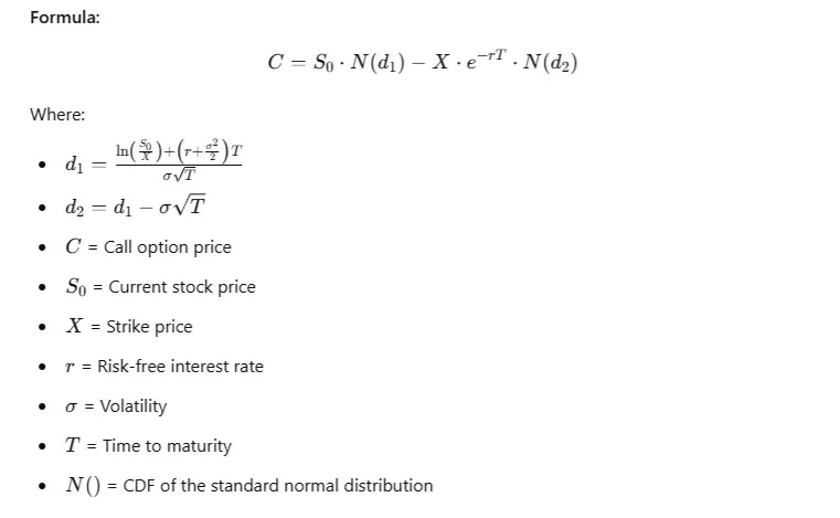
The Black-Scholes formula is used in finance to determine the price of European call and put options. It involves several mathematical functions, including the cumulative distribution function (CDF) of the standard normal distribution.

Python Code:

import math
from scipy.stats import norm

# Black-Scholes function to calculate call option price
def black_scholes_call(S0, X, T, r, sigma):
    d1 = (math.log(S0 / X) + (r + 0.5 * sigma ** 2) * T) / (sigma * math.sqrt(T))
    d2 = d1 - sigma * math.sqrt(T)
    call_price = S0 * norm.cdf(d1) - X * math.exp(-r * T) * norm.cdf(d2)
    return call_price

# Example values
S0 = 100  # Current stock price
X = 95    # Strike price
T = 1     # Time to maturity (1 year)
r = 0.05  # Risk-free interest rate
sigma = 0.2  # Volatility

print(f"Call Option Price: {black_scholes_call(S0, X, T, r, sigma):.2f}")

This function directly maps the formula into Python, using the math and scipy.stats libraries for mathematical operations and the normal CDF. It takes standard input parameters and outputs the option price in seconds.

2. Newton-Raphson Method for Finding Roots

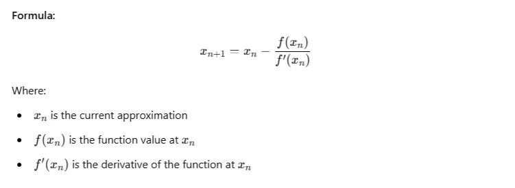
The Newton-Raphson method is a technique to find the root of a real-valued function. It’s iterative, making it useful for non-linear equations.

Python Code:

def newton_raphson(f, f_prime, x0, tolerance=1e-6, max_iterations=100):
    x_n = x0
    for n in range(max_iterations):
        fx_n = f(x_n)
        fpx_n = f_prime(x_n)
        if abs(fx_n) < tolerance:
            return x_n
        if fpx_n == 0:
            print("Zero derivative. No solution found.")
            return None
        x_n = x_n - fx_n / fpx_n
    print("Exceeded maximum iterations. No solution found.")
    return None

# Example function and its derivative
def func(x):
    return x**2 - 2  # Function f(x) = x^2 - 2

def func_prime(x):
    return 2 * x  # Derivative f'(x) = 2x

# Initial guess
initial_guess = 1.0

root = newton_raphson(func, func_prime, initial_guess)
print(f"Root of the function: {root}")

This function iterates using the Newton-Raphson formula. It keeps refining the guess until the function value is close to zero, indicating a root.

3. Fibonacci Sequence Using Matrix Exponentiation

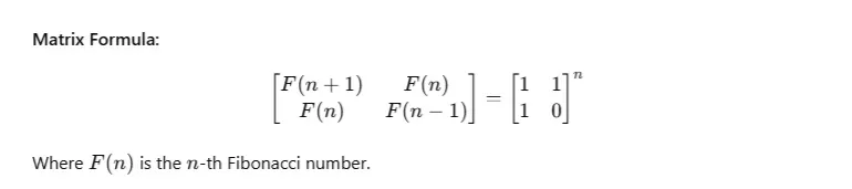
The Fibonacci sequence is a classic problem. Calculating Fibonacci numbers directly can be slow. Using matrix exponentiation, you can find the nnn-th Fibonacci number efficiently.

Python Code:

import numpy as np

# Function to calculate nth Fibonacci number using matrix exponentiation
def fibonacci_matrix(n):
    if n == 0:
        return 0
    F = np.array([[1, 1], [1, 0]], dtype=object)
    result = np.linalg.matrix_power(F, n - 1)
    return result[0][0]

# Example: Find the 10th Fibonacci number
n = 10
print(f"The {n}th Fibonacci number is: {fibonacci_matrix(n)}")

This approach uses NumPy to raise the Fibonacci matrix to the power nnn. It’s much faster than traditional methods, especially for large nnn.

4. Logistic Function for Population Growth

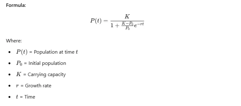
The logistic function models population growth with a carrying capacity.

Python Code:

import math

def logistic_growth(P0, K, r, t):
    return K / (1 + ((K - P0) / P0) * math.exp(-r * t))

# Example values
P0 = 50  # Initial population
K = 1000  # Carrying capacity
r = 0.1   # Growth rate
t = 10    # Time in years

population = logistic_growth(P0, K, r, t)
print(f"Population after {t} years: {population:.2f}")

This function calculates the population using the logistic growth model. It shows how a limited environment constrains growth over time.

Best Practices for Converting Mathematical Formulas into Python Code

Converting mathematical formulas into Python code can seem challenging at first, but by following a systematic approach, you can translate even complex equations into efficient and readable code. Below are the best practices to guide you through the process.

1. Understand the Formula Thoroughly

Before you begin coding:

• Identify Variables: Determine all the variables involved and their meanings.
• Recognize Constants: Note any constants and their values (e.g., π, e).
• Clarify Operations: Understand the mathematical operations used (addition, subtraction, multiplication, division, exponentiation, etc.).
• Know the Domains: Be aware of any constraints or domains of the variables (e.g., x≥0x \geq 0x≥0).

2. Break Down the Formula into Smaller Parts

Decompose the formula into manageable components:

• Compute Intermediate Values: Calculate parts of the formula separately.
• Simplify Complex Expressions: Break down complex expressions into simpler steps.

3. Map Mathematical Operations to Python Syntax

Translate mathematical operations to Python equivalents:

• Addition/Subtraction: +, -
• Multiplication/Division: *, /
• Exponentiation: ** or math.pow()
• Square Root: math.sqrt() or exponentiation with 0.5
• Constants: Use math.pi for π, math.e for e

4. Use Appropriate Libraries and Functions

Leverage Python’s standard libraries and external packages:

• math Module: For basic mathematical functions and constants.
• numpy Library: For array operations and advanced mathematical functions.
• scipy Library: For scientific computations and specialized functions.
• sympy Library: For symbolic mathematics (useful for symbolic calculations).​

5. Maintain the Order of Operations

Respect the mathematical precedence rules:

• Parentheses: Use parentheses to ensure operations are performed in the correct order.
• Operator Precedence: Remember that exponentiation has higher precedence than multiplication and division, which in turn have higher precedence than addition and subtraction.

6. Implement the Formula Step-by-Step:

Code the formula incrementally:

• Start Simple: Begin with the basic structure.
• Add Complexity Gradually: Incorporate additional components step by step.
• Use Variables for Intermediate Results: This improves readability and debuggability.

EXAMPLE:

import math

def quadratic_formula(a, b, c):
    # Calculate the discriminant
    discriminant = b ** 2 - 4 * a * c
    
    # Check for real solutions
    if discriminant < 0:
        return None  # No real roots
    
    # Calculate square root of discriminant
    sqrt_disc = math.sqrt(discriminant)
    
    # Compute two solutions
    x1 = (-b + sqrt_disc) / (2 * a)
    x2 = (-b - sqrt_disc) / (2 * a)
    
    return x1, x2

7. Test the Code with Known Values

Validate your implementation:

• Use Test Cases: Plug in values for which you know the expected result.
• Check Edge Cases: Test with boundary values to ensure robustness.
• Compare with Analytical Solutions: If possible, compare your results with analytical calculations or trusted tools.

8. Handle Special Cases and Errors

Anticipate and manage potential issues:

• Domain Errors: Check for invalid inputs (e.g., division by zero, negative values under a square root).
• Exception Handling: Use try and except blocks where appropriate.
• Return Meaningful Messages: Provide clear feedback when errors occur.

Consult resources:

• Python Documentation: For built-in functions and modules.
• Library References: Such as NumPy and SciPy documentation.
• Mathematical References: To confirm formulas and understand their derivations.

Common Mathematical Functions in Python

When converting mathematical formulas into Python code, knowing where to find and how to use common mathematical functions is essential. Python provides a rich set of libraries that include a wide range of mathematical functions, from basic arithmetic to complex statistical computations. Below, we’ll explore the primary libraries and functions you’ll frequently use when translating mathematical formulas into Python code.

The math Module

The built-in math module provides access to many basic mathematical functions:

Arithmetic Functions:

• math.sqrt(x): Returns the square root of x.
• math.exp(x): Returns the exponential of x (eˣ).
• math.log(x[, base]): Returns the logarithm of x to the specified base. Defaults to natural logarithm (base e) if the base isn’t specified.
• math.pow(x, y): Returns x raised to the power y (xʸ).

Trigonometric Functions:

• math.sin(x): Returns the sine of x radians.
• math.cos(x): Returns the cosine of x radians.
• math.tan(x): Returns the tangent of x radians.
• math.asin(x), math.acos(x), math.atan(x): Inverse trigonometric functions.

Constants:

• math.pi: Mathematical constant π (pi).
• math.e: Mathematical constant e.

Additional Arithmetic Functions:

math.ceil(x): Returns the smallest integer greater than or equal to x (i.e., rounds x upward to an integer).

math.floor(x): Returns the largest integer less than or equal to x (i.e., rounds x downward to an integer).

math.trunc(x): Returns the integer part of x, removing any fractional digits.

math.fabs(x): Returns the absolute value of x as a floating-point number.

math.modf(x): Returns the fractional and integer parts of x as a tuple. Both parts have the same sign as x.

math.fmod(x, y): Returns the modulo of x and y (remainder of division), following the platform C library.

math.gcd(a, b): Returns the greatest common divisor of the integers a and b.

math.lcm(a, b): Returns the least common multiple of the integers a and b. (Added in Python 3.9)

math.factorial(x): Returns the factorial of x, an exact integer.

math.isqrt(n): Returns the integer square root of the non-negative integer n. (Added in Python 3.8)

math.comb(n, k): Returns the number of ways to choose k items from n items without repetition and without order (i.e., combinations). (Added in Python 3.8)

math.perm(n, k=None): Returns the number of ways to choose k items from n items without repetition and with order (i.e., permutations). If k is None, it returns math.factorial(n). (Added in Python 3.8)

Hyperbolic Functions:

math.sinh(x): Returns the hyperbolic sine of x.

math.cosh(x): Returns the hyperbolic cosine of x.

math.tanh(x): Returns the hyperbolic tangent of x.

math.asinh(x): Returns the inverse hyperbolic sine of x.

math.acosh(x): Returns the inverse hyperbolic cosine of x (for x ≥ 1).

math.atanh(x): Returns the inverse hyperbolic tangent of x (for -1 < x < 1).

Angle Conversion Functions:

math.degrees(x): Converts angle x from radians to degrees.

math.radians(x): Converts angle x from degrees to radians.

Distance and Coordinate Functions:

math.hypot(*coordinates): Returns the Euclidean norm (hypotenuse) of a vector, i.e., the square root of the sum of squares of its components.

math.dist(p, q): Returns the Euclidean distance between two points p and q, each given as a sequence of coordinates. (Added in Python 3.8)

Special Functions:

math.gamma(x): Returns the Gamma function at x.

math.lgamma(x): Returns the natural logarithm of the absolute value of the Gamma function at x.

math.erf(x): Returns the error function at x.

math.erfc(x): Returns the complementary error function at x, defined as 1 - math.erf(x).

math.expm1(x): Returns eˣ - 1. For small x, this function gives a more precise result than math.exp(x) - 1.

math.log1p(x): Returns the natural logarithm of 1 + x. For small x, this function gives a more precise result than math.log(1 + x).

Comparison and Testing Functions:

math.isclose(a, b, *, rel_tol=1e-09, abs_tol=0.0): Determines whether two values a and b are close to each other, within a specified tolerance.

math.isfinite(x): Returns True if x is neither infinity nor NaN (Not a Number).

math.isinf(x): Returns True if x is positive or negative infinity.

math.isnan(x): Returns True if x is NaN.

Constants:

math.tau: The mathematical constant τ (tau), equivalent to 2π (approximately 6.283185307179586).

math.inf: A floating-point positive infinity.

math.nan: A floating-point “Not a Number” (NaN) value.

Logarithmic Functions:

math.log2(x): Returns the base-2 logarithm of x.

math.log10(x): Returns the base-10 logarithm of x.

Rounding Functions:

math.copysign(x, y): Returns a float with the magnitude (absolute value) of x and the sign of y.

math.fsum(iterable): Returns an accurate floating-point sum of values in the iterable. It avoids loss of precision by tracking multiple intermediate partial sums.

Examples of Using the math Module

Example 1: Calculating Compound Interest

import math

def compound_interest(principal, rate, times_compounded, years):
    # A = P * (1 + r/n)^(n*t)
    amount = principal * math.pow((1 + rate / times_compounded), times_compounded * years)
    return amount

# Usage
initial_amount = 1000
annual_rate = 0.05
compounded_times = 12
investment_period = 10

final_amount = compound_interest(initial_amount, annual_rate, compounded_times, investment_period)
print(f"Final amount after {investment_period} years: ${final_amount:.2f}")

Example 2: Solving a Quadratic Equation

import math

def solve_quadratic(a, b, c):
    # ax^2 + bx + c = 0
    discriminant = math.pow(b, 2) - 4 * a * c
    if discriminant >= 0:
        root_disc = math.sqrt(discriminant)
        x1 = (-b + root_disc) / (2 * a)
        x2 = (-b - root_disc) / (2 * a)
        return x1, x2
    else:
        return None  # No real roots

# Usage
roots = solve_quadratic(1, -3, 2)
if roots:
    print(f"The roots are: {roots[0]} and {roots[1]}")
else:
    print("No real roots")

Thank you for following along with this tutorial. We hope you found it helpful and informative. If you have any questions, or if you would like to suggest new Python code examples or topics for future tutorials/articles, please feel free to join and comment. Your feedback and suggestions are always welcome!

You can find the same tutorial on Medium.com.